
Loading cart contents...
Ilustrating Lagrangian Variables
In the last post we had a tentative on Variational Mechanics which resulted very stimulating.
In order settle ideas down, I have left the subject cooling in the fridge and I have fiddled around with the Lego Mindstorms(c) robot we have at the RGEX research group, trying to make a positioning system that is accurate enough for our purposes.
Surely Jaume (my thesis director) will be very happy to hear about it.
I know this is not the exact place for it, but it’s my blog and I do what I want to…hehehe…anyway, whoever wants to see what we do there, it is available at: www.rgex.blogspot.com.
And now, back to work:
The intention of this post it to illustrate some relationships that exist in Mechanics and that are repeated ad-vomitum in every reference one finds on Variational Mechanics.
The main problem I have encountered is that explanations mix numerical methods with physical concepts, and more often that seldom everything is written in the cryptic language of mathematicians. Of course, in complete absence of figures or anything of the like.
So, here we go…
With the help of some coding in C++ and QtOctave (https://forja.rediris.es/projects/csl-qtoctave/), I have made some graphics for the simulation of a moving particle.
I have used the same deductive principle I have seen in the papers, which is not intuitive at all. Hopefully some drawings will make it more clear.
A moving particle
Instead of trying to obtain the formula in a straightforward manner, the Least Action Principle suggest one to imagine an arbitrary particle that changes its position from one place to another. So, that’s exactly what I have done.
The code iterates some 100 times and assigns random values to the new position of our particle. Really simple stuff.

The red dots represent all 100 different positions the particle goes when random increments in x and y are applied.
The initial point is at (10,10), and all the following are dQ further (dQ is divided in X and Y components, of course). dQ gets a random value for each iteration.
Once we have the new positions, it is straightforward to apply physics concepts to get the values of Velocity, Acceleration, Kinetic Energy and Potential Energy that have to be applied to get the particle there:
V=dQ/dt
A=dV/dt
Ep=m*A*dQ
Ec=1/2(m*|V|²)
With a dt value of 0.1 and a mass m of 5, it is also a piece of cake to obtain a table with the respective values.
Work and energy
The magnitudes Work and Energy are directly related to the Ep and Ec values.
From a physical point of view, there are some very interesting things that can be observed when putting their values against the |dQ| values:

Distance |dQ| vs kynetic energy Ec
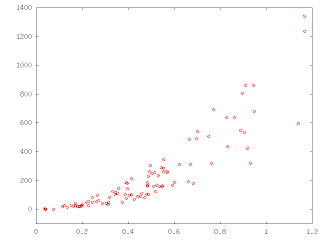
Distance |dQ| vs potential energy Ep
From the same experiment, the random values of distance show a correlation of two types with the respective energies:
- Kynetic energy is linearly related to the distance covered by the particle. Its values depend solely on the module of the velocity parameter, which itself is linearly dependent on the distance.
- Potential energy shows a more quadratic behaviour, provided its acceleration component is multiplied by the covered distance.
It is also interesting to have a look at the graph Ec vs Ep, where also the quadratic behaviour is observed:

Kynetic energy Ec vs Potential energy Ep
Interestingly enough, both (|dQ| vs Ep) and (Ec vs Ep) are exactly the same shape, but for the scale of the X axis, which is of course linearly related.
The basic variational principle
The following step once these observations are made, is that of nesting our little freely moving particle loop into another broader loop, and accumulate the values of the position to form a trajectory.
Provided the inner loop generates a bunch of 100 probable future positions, one tempting criterion would be to choose that of minimum value for the total calculated energy…

The random accumulated trajectory of the particle
Just to verify that by adding the minimum energy substeps we still get a random trajectory.
Obviously, no constraints have been applied, and the particle represents a «Markov process».
What the basic variational principle teachs us is that, given certain constraints, the trajectory of the particle would have been that of minimum energy.
In our code for each time step the chosen subpath has been that of minimum energy.
Nonetheless, for the global trajectory, i.e. after a series of timesteps, a more holistic approach has to be taken in order to obtain the actual «natural» path.
That is the ODEs approach, and we’ll talk about it in further episodes…
Nonetheless, for the global trajectory, i.e. after a series of timesteps, a more holistic approach has to be taken in order to obtain the actual «natural» path.
That is the ODEs approach, and we’ll talk about it in further episodes…
The following is the C++ code employed to obtain the tables. These have been plotted with QTOctave, an opensource version of MathLab.
Please note that it is the version which provides the complete path. The inner loop provides the random new positions and the outer loops concatenates one position after another, selecting each time that with the minimum energy.
main.cpp:
Conoce el programa, la nueva metodología de diseño: "Co-Creación Procedural"
Clic aqui si quieres entender como generar sinergías entre algoritmos, diseñadores y empresas para crear nuevos productos y servicios que generan ingresos pasivos. ¿Te quedarás atrás?, otros ya están usando el poder de los algoritmos y co-creando con ellos. ⇱